Managing Fantasy World Maps in GDAL
The benefit of using GDAL to manage a world map with GDAL is that you are not limited by resolution like you would be with G.Projector. You can make your map as detailed as possible, and GDAL should be able to handle it, as long as your computer can.
Disclaimer: Everything I do with GDAL on the command line you can absolutely do with QGIS. I’m a software engineer by trade, though, so I’m at home on the command line.
Disclaimer 2: I am not a GIS expert, so if anything I say in this post sounds completely wrong, please don’t hesitate to let me know :)
GDAL Version
I use GDAL version 3.2. You need at least GDAL version 3.1 to run the commands I run in this tutorial, since the -a_ulurll command is only available in 3.1+
Equirectangular Map
Your “source of truth” is your equirectangular map. My process starts with an landmask equirectangular world map, white=land and black=ocean.
The plan is to reproject our equirectangular map in different ways to reduce distortion for finalizing the coastlines and building the heightmap. Working with as little distortion as possible makes it easier to create the heightmap, figure out rivers, and more. Getting an entire landmass relatively distortion-free becomes much harder if your landmass is huge, and this is personally something I have not tackled yet. My main world is half the radius of earth, and probably 85+% water, so my landmasses are relatively small and easy to capture in a single projection.
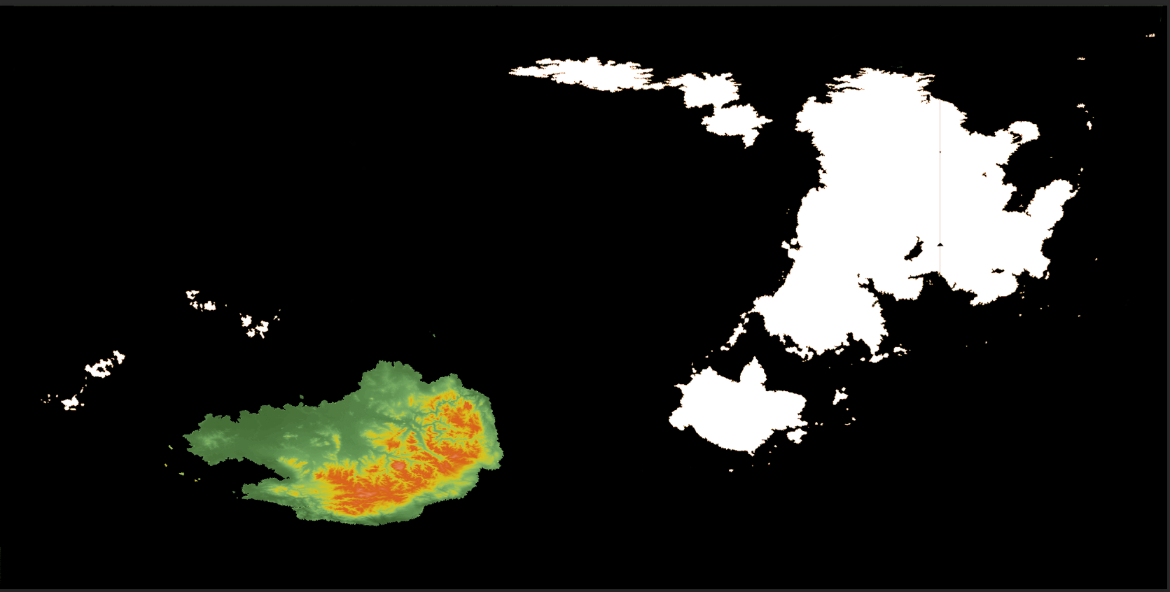
For this tutorial, I’ll be using a new world map:
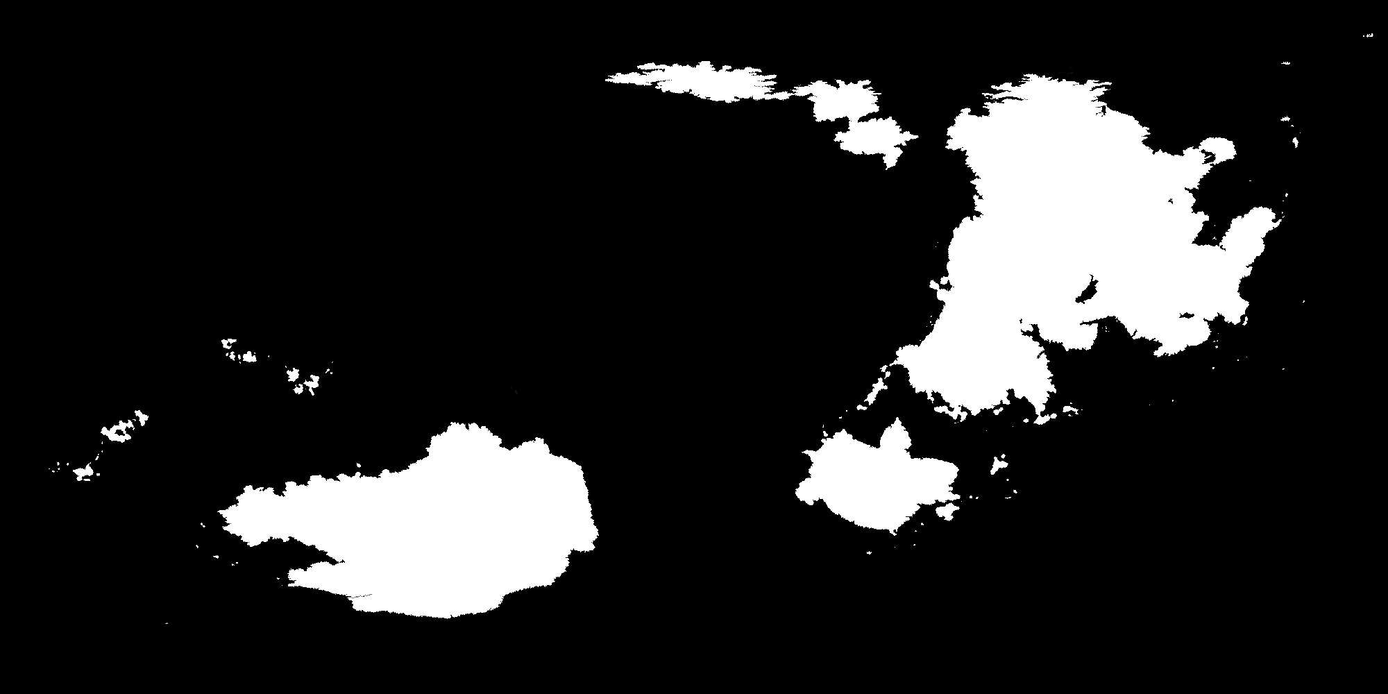
I’ll work with the lower left continent for now.
Adding Geo Referencing to the Equirectangular World Map
First, we need to add geo-referencing information to our base map. To do this, run the command:
gdal_edit.py -a_srs EPSG:4326 -a_ullr -180 90 180 -90 map.tif
EPSG:4326 is basically the “plate caree” or equirectangular projection. the numbers define the extents of the projection.
Figuring out projection parameters
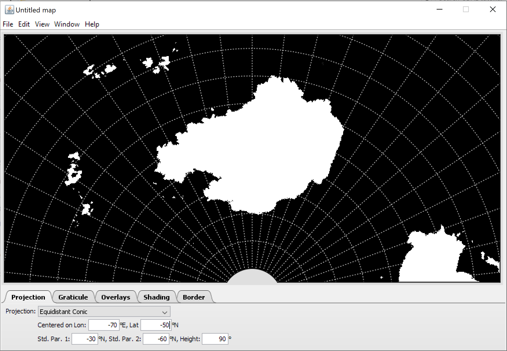
The easiest way to figure out what exactly you want to project to is to use G.Projector. I will create a lower resolution version of my equirectangular map, usually 6000x3000 or so, in png format.
Loading that up into G.Projector and playing with the settings, I end up with a equidistant conic projection that looks like this:
Reprojecting to Equidistant Conic
This web page: http://geotiff.maptools.org/proj_list/ has a master list of the project codes for pretty much all projections that GDAL can do.
To reproject our base map, we want to use the gdal_warp command. Setting up our equidistant projection looks like this:
gdalwarp -t_srs "+proj=eqdc +lat_1=-30 +lat_2=-60 +lon_0=-70" -r mode map.tif equidistant_conic.tif
Depending on the resolution of your map, this will take awhile.
Once complete, you can run gdalinfo equidistant_conic.tif to see the new georeferencing information:
Driver: GTiff/GeoTIFF
Files: equidistant_conic.tif
Size is 8760, 6947
Coordinate System is:
PROJCRS["unknown",
    BASEGEOGCRS["WGS 84",
        DATUM["World Geodetic System 1984",
            ELLIPSOID["WGS 84",6378137,298.257223563,
                LENGTHUNIT["metre",1]]],
        PRIMEM["Greenwich",0,
            ANGLEUNIT["degree",0.0174532925199433]],
        ID["EPSG",4326]],
    CONVERSION["Equidistant Conic",
        METHOD["Equidistant Conic"],
        PARAMETER["Latitude of natural origin",0,
            ANGLEUNIT["degree",0.0174532925199433],
            ID["EPSG",8801]],
        PARAMETER["Longitude of natural origin",-70,
            ANGLEUNIT["degree",0.0174532925199433],
            ID["EPSG",8802]],
        PARAMETER["Latitude of 1st standard parallel",-30,
            ANGLEUNIT["degree",0.0174532925199433],
            ID["EPSG",8823]],
        PARAMETER["Latitude of 2nd standard parallel",-60,
            ANGLEUNIT["degree",0.0174532925199433],
            ID["EPSG",8824]],
        PARAMETER["False easting",0,
            LENGTHUNIT["metre",1],
            ID["EPSG",8806]],
        PARAMETER["False northing",0,
            LENGTHUNIT["metre",1],
            ID["EPSG",8807]]],
    CS[Cartesian,2],
        AXIS["easting",east,
            ORDER[1],
            LENGTHUNIT["metre",1,
                ID["EPSG",9001]]],
        AXIS["northing",north,
            ORDER[2],
            LENGTHUNIT["metre",1,
                ID["EPSG",9001]]]]
Data axis to CRS axis mapping: 1,2
Origin = (-21227652.971526119858027,10001965.729313574731350)
Pixel Size = (4846.117353881320014,-4846.117353881320014)
Metadata:
  AREA_OR_POINT=Area
  TIFFTAG_DATETIME=2020:07:23 11:35:30
  TIFFTAG_RESOLUTIONUNIT=2 (pixels/inch)
  TIFFTAG_SOFTWARE=Adobe Photoshop 21.0 (Windows)
  TIFFTAG_XRESOLUTION=72
  TIFFTAG_YRESOLUTION=72
Image Structure Metadata:
  INTERLEAVE=PIXEL
Corner Coordinates:
Upper Left  (-21227652.972,10001965.729) (134d21'23.00"W,169d 3'49.28"N)
Lower Left  (-21227652.972,-23664011.528) (117d51'16.66"E,120d14'19.24"N)
Upper Right (21224335.048,10001965.729) (  5d39' 0.05"W,169d 2'32.92"N)
Lower Right (21224335.048,-23664011.528) (102d 9' 3.46"E,120d12'46.74"N)
Center      (   -1658.962,-6831022.899) ( 70d 1'51.34"W, 61d35'16.99"S)
Band 1 Block=8760x1 Type=Byte, ColorInterp=Red
Band 2 Block=8760x1 Type=Byte, ColorInterp=Green
Band 3 Block=8760x1 Type=Byte, ColorInterp=Blue
Reprojecting back to Equirectangular
Inevitably, you will be editing this equidistant conic map in Photoshop or other photo editing/terrain editing software. Throughout this process, your tif file will lose the georeferencing information, since when you save in these programs, they don’t know to retain that metadata. What I would recommend is to, when making edits, save to a new file. For instance, equidistant_conic_heightmap.tif. That way, you can go back and reference your original georeferencing data in equidistant_conic.tif.
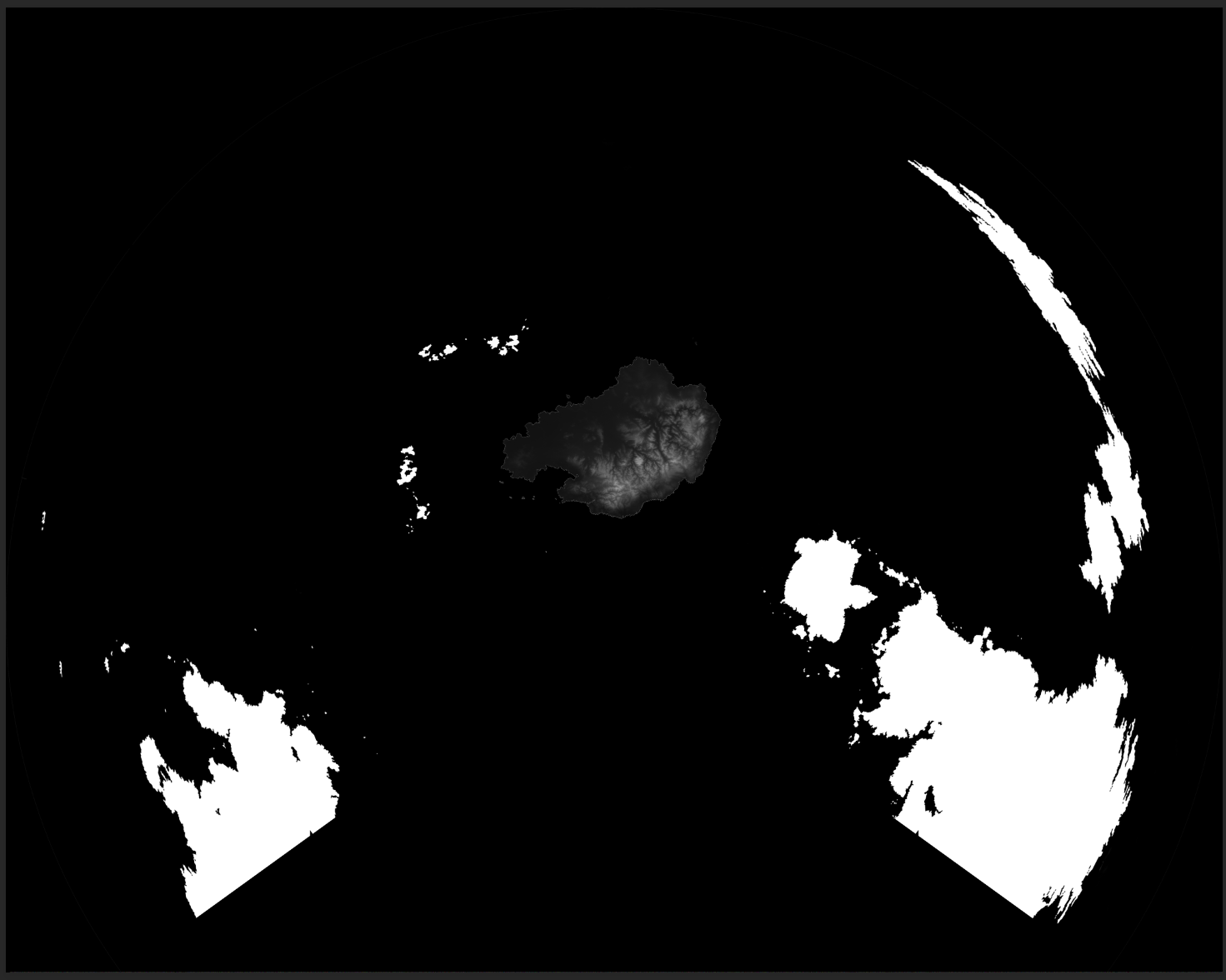
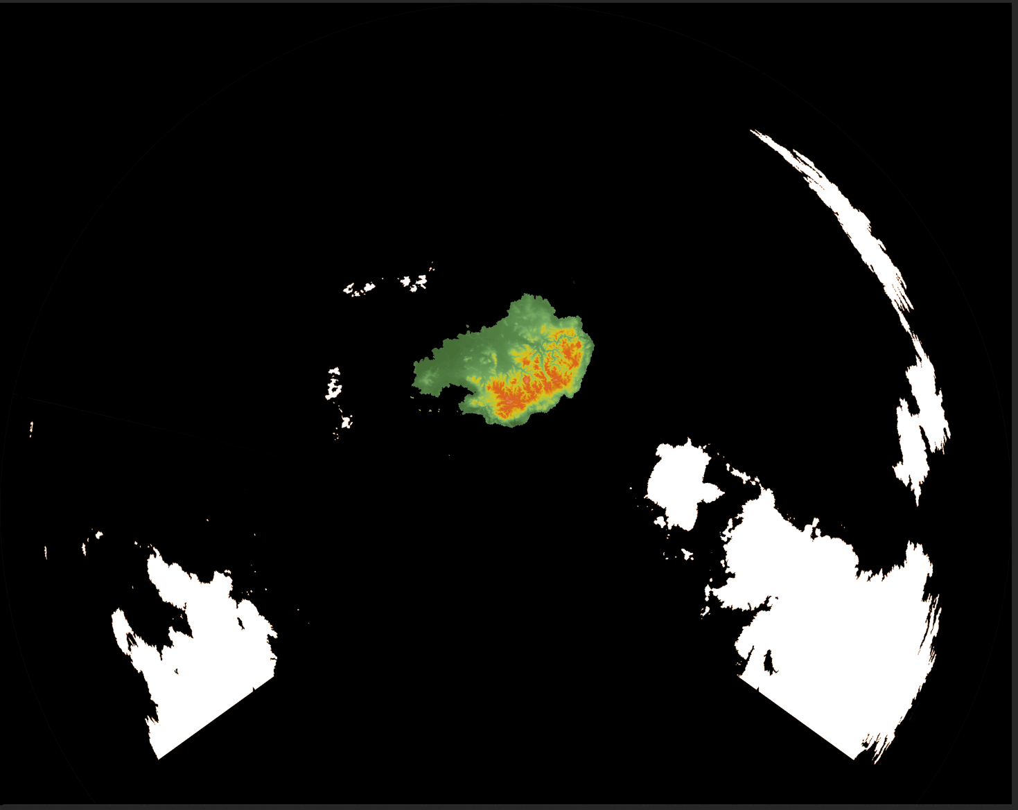
Note: This post is not covering heightmap creation, yet. I just pasted a bit of the australia map from the last post. The scale is not even close.
Once we have a new map ready to reproject back to equirectangular, we will need to add back the georeferencing information. We need to set the type of projection and associated information, along with the corner coordinates, which defines the extents of the map. You can find this information using gdalinfo like we did in the last section.
For the a_ulurll* command, we are giving “upper left”, “upper right”, “lower left”. We need to use this parameter instead of the standard -a_ullr command since the equidistant conic projection is not square (it’s probably more complicated then that, but that’s my rudimentary understanding). p
*this is the option that is only available in 3.1+, and we need it!
gdal_edit.py -a_srs "+proj=eqdc +lat_1=-30 +lat_2=-60 +lon_0=-70" -a_ulurll -21227652.972 10001965.729 21224335.048 10001965.729 -21227652.972 -23664011.528 equidistant_conic_heightmap.tif
With the georeferencing data added back in, we can reproject back to equirectangular:
gdalwarp -t_srs EPSG:4326 -r mode equidistant_conic_heightmap.tif equirectangular_final.tif

The plan is to follow a similar process for each continent, then combine each equirectangular map into a single master file. The great thing about this process is that you can do it at as high of a resolution as you want. Fair warning, though, gdalwarp operations can take a long time at really high resolutions, especially with a 16-bit image.